CS 180 Portfolio

We used the pretrained DeepFloyd diffusion to run some tests. The interesting thing here is that we can change the detail at which these pictures are made with the number of inference steps. Here are two examples. The random seed I am using is 4.

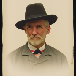
man with a hat (inference 20)

rocket (inference 20)

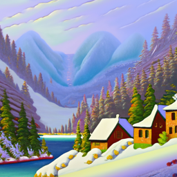
oil painting of a snowy village (inference 20)

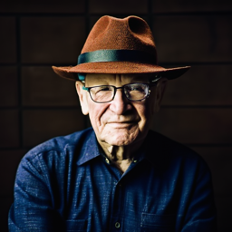
man with a hat (inference 40)

rocket (inference 40)

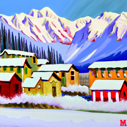
oil painting of a snowy village (inference 40)

As we can see, the higher the inference, the more detail we get. This is best seen in the man with the hat, where there are more wrinkles and details on the shirt.

The first step we did is to add noise to our image. The way we did this is through an equation, x_t = sqrt(a_t)x_0 + sqrt(1 - a_t)e, where e is sampled from a gaussian. Here, we have the image sampled at 3 different t's: 250, 500, 750.

Berkeley Campanile

t = 250

t = 500

t = 750

As we can see, the higher the t, the more noisy the image.

Now, we'll try using classical methods, such as Gaussian blur filtering. This is just using the standard torchvision gaussian blur.

t = 250

t = 500

t = 750

t = 250, gaussian blur denoised

t = 500, gaussian blur denoised

t = 750, gaussian blur denoised

As we can see, the results are not so great.

Now, we'll use one step denoising to try and denoise it better. The way we'll do this is using the pretrained UNet thorugh using our equation from earlier, where the UNet will predict the error.

t = 250

t = 500

t = 750

t = 250, One step denoised

t = 500, One step denoised

t = 750, One step denoised

As we can see, this is a much better result than when classical methods.

Now, we'll try iterative denoising. Instead of trying to just guess the noise in one step, we'll try to get an estimate of a previous timestep, and predict that. The way we would do that is through another mathematical formula: x_t_prime = sqrt(a_bar_t_prime) B_t / (1 - a_bar_t) * x_0 + sqrt(a_t)(1 - a_bar_t_prime) / (1 - a_bar_t) x_t + v_sigma, where v_sigma is a random noise that the model predicts.

t = 90

t = 240

t = 390

t = 540

t = 690

Berkeley Campanile

Iteravely denoised

One step denoised

t = 750, gaussian blur denoised

Here, we the image at different steps. As the final results show, the iteratively denoised has the best results and closest to original.

Now, we'll input pure noise into the model, and see what the model generates from that.

Sample 1

Sample 2

Sample 3

Sample 4

Sample 5

These are some pretty cool things that the model generated from pure noise!

The generated pictures can be improved by using Classifier Free Guidance. This means that we can we compute both a conditional and unconditional noise estimate, and by combining the two, we will get better pictures! We used a gamma value of 7

Sample 1

Sample 2

Sample 3

Sample 4

Sample 5

As we can see, the pictures generated are definitely better than what we had earlier.

Now, we use the iterative denoising function with CFG to generate images that are close to our source image by take our original image, injecting a little bit of gaussian noise, then specifying different t values to start at. As we can see, the later the t value, then the closer we get to our original image.

i_start = 1

i_start = 3

i_start = 5

i_start = 7

i_start = 10

i_start = 20

original photo

i_start = 1

i_start = 3

i_start = 5

i_start = 7

i_start = 10

i_start = 20

original photo

i_start = 1

i_start = 3

i_start = 5

i_start = 7

i_start = 10

i_start = 20

original photo

Here are two different images that I chose on my own, I chose the empire state building and the great wall of china. I wanted to see how well it could capture the details.

So now we try using nonrealistic images. I tried a few different images, including an online image of an anime character, as well as two and drawn images.

i_start = 1

i_start = 3

i_start = 5

i_start = 7

i_start = 10

i_start = 20

original photo

i_start = 1

i_start = 3

i_start = 5

i_start = 7

i_start = 10

i_start = 20

original photo

i_start = 1

i_start = 3

i_start = 5

i_start = 7

i_start = 10

i_start = 20

original photo

i_start = 1

i_start = 3

i_start = 5

i_start = 7

i_start = 10

i_start = 20

original photo

One interesting thing to note is that the image did not do well with the text within my image.

The next test we did is to see if the model can paint in parts that we remove. For example, if we tkae a block outside of the campanile, what would the model produce?

original

mask

hole to fill

result

original

mask

hole to fill

result

original

mask

hole to fill

result

These are some pretty interesting results!

Now, we'll give it a text condition, but input our original image with some noise to see how the model can try to get to our desired text.

i_start = 1

i_start = 3

i_start = 5

i_start = 7

i_start = 10

i_start = 20

original photo

i_start = 1

i_start = 3

i_start = 5

i_start = 7

i_start = 10

i_start = 20

original photo

i_start = 1

i_start = 3

i_start = 5

i_start = 7

i_start = 10

i_start = 20

original photo

These are some very interseting pictures!

Now, we'll try to have visual anagrams. This means that when we have it upright, the picture will look one way, and if we flip the picture, it'll look like something else. The way we did this is by adding two different noises. One would be the first image we chose. Then, we would flip the image, generate the noise given the second prompt, then flip it again. Then we would average these two noises to get the next timestep

People around a campfire

Oil painting of a man

Photo of a man

Photo of a dog

Coast of amalfi

Hipster person

These are some really cool applications of the stuff we worked on. The only one that didn't work out super well was the dog/human, but i feel like that is because it's hard to merge the two.

Finally, we'll implement hybrid images by creating another composite noise. The way this will work is if we combine the low frequencies of one noise with the high frequencies of another.

Skull/Waterfall

Oil painting of snow maountains/waterfalls

Rocket Pencil

Now, we'll try to actually build our own UNET denoiser, using an L2 loss. The way we trained it is similar to how we did earlier: by adding gaussian noise to our pictures. Then, we'll train it using an Adam optimizer. Here's how they look after a few epochs of training

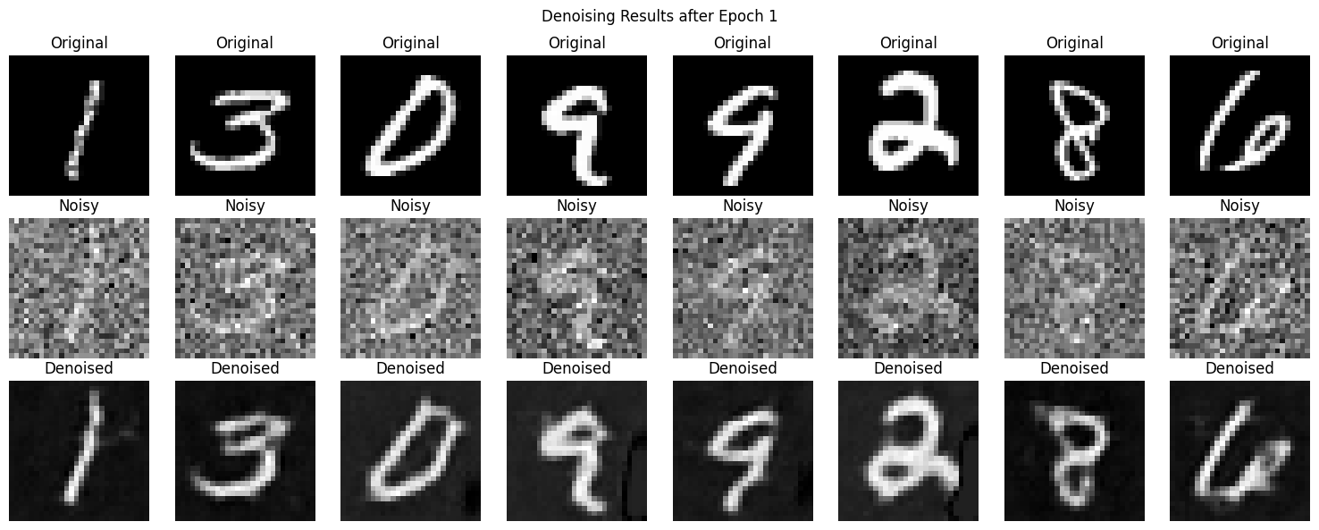
Results after epoch 1

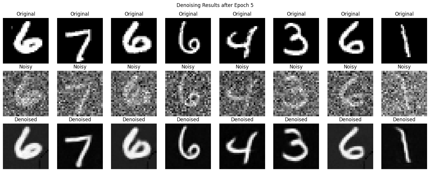
Results after epoch 5

Below is a graph of the loss.

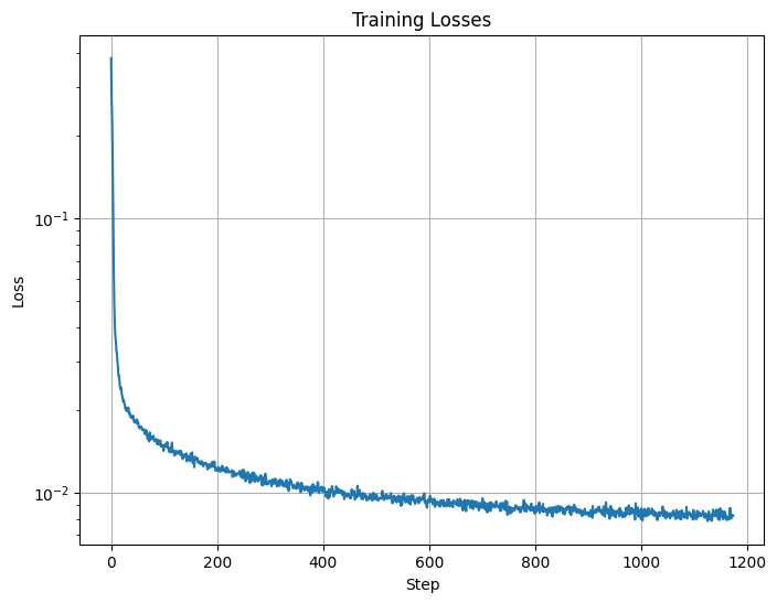
Loss

Now, we'll see what the denoised output is for varying levels of noise.

sigma = 0

sigma = 0.2

sigma = 0.4

sigma = 0.5

sigma = 0.6

sigma = 0.8

sigma = 1.0

Now, we'll try to inject a scalar t into our unet to condition it on time. The way we will do this is to add it in in between our up blocoks, and add to the result from what we had. Here is the resulting loss curve plot for the time conditioned UNet

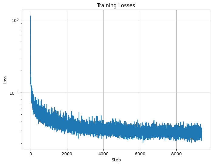
Loss

Here are the results of the sampling from epoch 5 and epoch 20.

Results after epoch 5

Results after epoch 20

Now, we'll do something similar but add class conditioning. Here is the resulting loss curve.

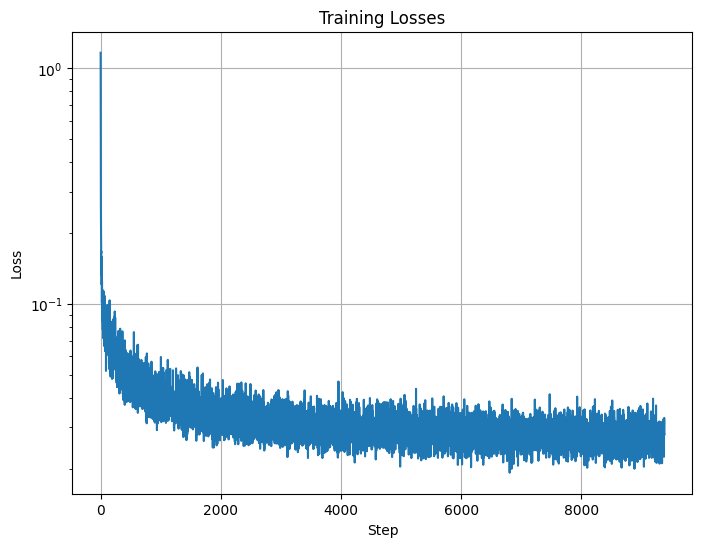
Loss

Here are the results of the sampling from epoch 5 and epoch 20.

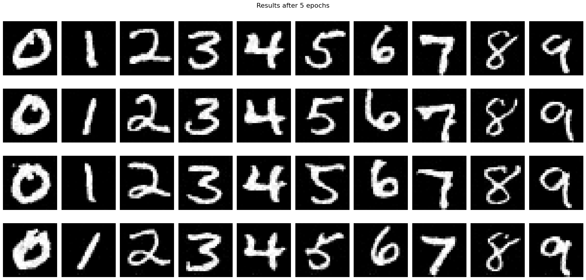
Results after epoch 5

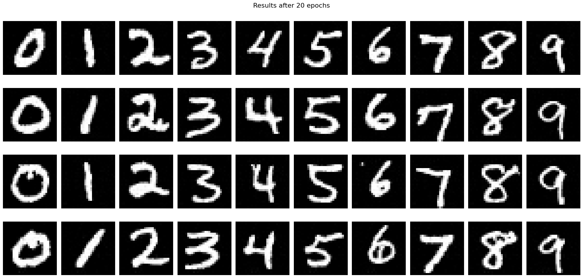
Results after epoch 20